SMART processing example.

SMART processing example from the creation of the first map to the extraction of it’s properties.

from matplotlib import pyplot as plt

from sunpy.map import Map

from smart.calculate_properties import cosine_weighted_area_map, dB_dt, extract_features, get_properties
from smart.differential_rotation import diff_rotation
from smart.indexed_grown_mask import index_and_grow_mask, plot_indexed_grown_mask
from smart.processing import (
    calculate_cosine_correction,
    cosine_correct_data,
    map_threshold,
    smart_prep,
    smooth_los_threshold,
)

Data Preparation

We start by creating a sunpy.Map from our .fits file.

hmi_map = Map("http://jsoc.stanford.edu/data/hmi/fits/2024/06/06/hmi.M_720s.20240606_230000_TAI.fits")
# hmi_map = Map(
#     "https://solmon.dias.ie/data/2024/06/06/HMI/fits/hmi.m_720s_nrt.20240606_230000_TAI.3.magnetogram.fits"
# )

We’ll also plot this map to see how it looks before applying any of the SMART processes.

hmi_map.plot()

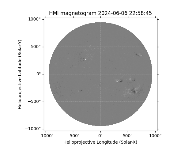
<matplotlib.image.AxesImage object at 0x7ff1d15f05b0>

We apply the map_threshold function, which sets the off-disk pixels to nans, makes them black, and also clips the map data. We’ll plot this new thresholded map to see how it looks.

thresholded_map = map_threshold(hmi_map)
thresholded_map.plot()

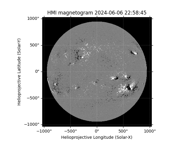
<matplotlib.image.AxesImage object at 0x7ff1d1659420>

Next we’ll use the smooth_los_threshold function in order to get a smoothed version of our map. This will then be used with the calculate_cosine_correction and cosine_correct_data functions to get cosine corrected data for our map

Once again we will use a plot to see how our corrected data looks.

smooth_map, filtered_labels, mask_sizes = smooth_los_threshold(thresholded_map)
cos_correction = calculate_cosine_correction(smooth_map)
corrected_data = cosine_correct_data(smooth_map, cos_correction)
plt.imshow(corrected_data.value)

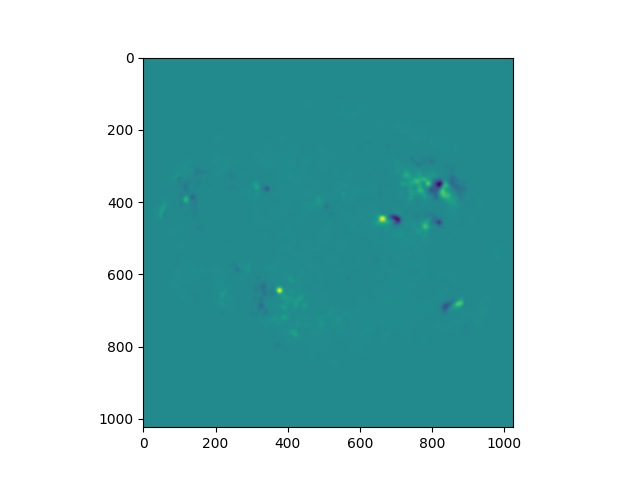
<matplotlib.image.AxesImage object at 0x7ff1d14944f0>

We now need to prepare our second map, taken from a time ‘Δt’ before the first.

This time we’ll simply use the smart_prep function to create our thresholded map and calculate the corrected data. This function performs the smooth_los_threshold, calculate_cosine_correction, and cosine_correct_data functions.

hmi_map_prev = Map("http://jsoc.stanford.edu/data/hmi/fits/2024/06/06/hmi.M_720s.20240606_000000_TAI.fits")
# hmi_map_prev = Map(
#     "https://solmon.dias.ie/data/2024/06/06/HMI/fits/hmi.m_720s_nrt.20240606_000000_TAI.3.magnetogram.fits"
# )
thresholded_map_prev, cos_correction_prev = smart_prep(hmi_map_prev)

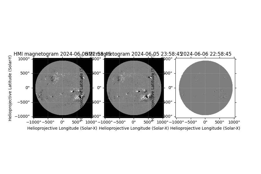
We will now differentially rotate our second, earlier, map to the time, ‘t’, of our original map. We will use the diff_rotation function to do this. Later this rotated map will be useful for removing transient features from our masks.

We plot the three maps. From left to right we have our map from time ‘t’, our map from time ‘t - Δt’, and finally our rotated map.

rotated_map = diff_rotation(hmi_map, hmi_map_prev)
diff_map = Map((hmi_map.data - rotated_map.data, rotated_map.meta))
fig, ax = plt.subplot_mosaic(
    [["cur", "prev", "diff"]],
    figsize=(9, 6),
    per_subplot_kw={
        "cur": {"projection": hmi_map},
        "prev": {"projection": hmi_map_prev},
        "diff": {"projection": rotated_map},
    },
)
hmi_map.plot(axes=ax["cur"])
hmi_map_prev.plot(axes=ax["prev"])
diff_map.plot(axes=ax["diff"])

<matplotlib.image.AxesImage object at 0x7ff1d1405ed0>

Region Detection

Now that we have our map from time ‘t’ and the map rotated to time ‘t’, we can subtract them in order to remove any transient features due to solar rotation.

The index_and_grow_mask function performs this operation, and also orders the detected active regions in order of descending area, and assigns an ascending integer value to these regions, starting with 1.

sorted_labels = index_and_grow_mask(hmi_map, rotated_map)

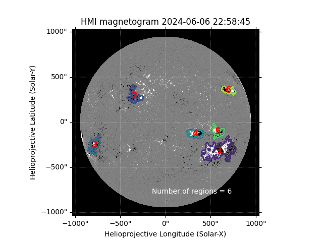
Using the plot_indexed_grown_mask function we can easily see how the map now looks with it’s contours and region labels.

plot_indexed_grown_mask(hmi_map, sorted_labels)

Characterization

The extract_features function returns an array of individual feature masks for each detected region. The cosine_weighted_area_map is used to return a cosine corrected area map of the disk, which is later used in combination with the aforementioned feature masks in order to extract properties from individual regions.

feature_masks = extract_features(sorted_labels)
region1_feature_mask = feature_masks[:1]
region1_area_map = cosine_weighted_area_map(hmi_map)

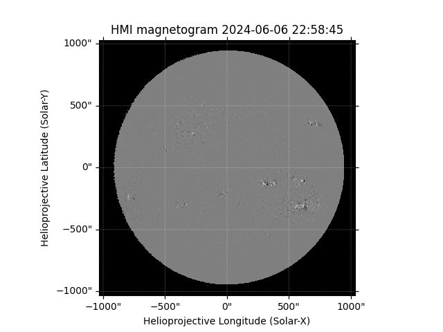
We will call the dB_dt function and plot the result in order to see a map showing the temporal change of the magnetic field on the solar disk.

dBdt, dt = dB_dt(hmi_map, hmi_map_prev)
dBdt.plot()

<matplotlib.image.AxesImage object at 0x7ff1d146c850>

Finally, we use our get_properties function to extract information relating to the magnetic field strength, flux, and area of each identified active region.

properties = get_properties(hmi_map, dBdt, dt, sorted_labels)

for i in range(len(properties)):
    for prop, value in properties[i].items():
        print(prop, ":", value)
    print()

feature label : 1
flux emergence rate : 827.3424378920586 Wb / s
mean B : 0.3138936626971728 G
std B : 24.452945786497033 G
minimum B : -1068.5 G
maximum B : 1247.8000000000002 G
positive flux : 177288539080923.62 Wb
negative flux : -129515858814029.11 Wb
unsigned flux : 306804397894952.75 Wb
flux imbalance : 6.422172592806393
total area (millionths) : 9130.873555891341

feature label : 2
flux emergence rate : -304.62129596472585 Wb / s
mean B : -0.07426020437685889 G
std B : 14.54994365208442 G
minimum B : -551.9 G
maximum B : 1932.8000000000002 G
positive flux : 26759921477710.164 Wb
negative flux : -38061866759999.0 Wb
unsigned flux : 64821788237709.164 Wb
flux imbalance : -5.73545408499639
total area (millionths) : 2277.8357622914323

feature label : 3
flux emergence rate : -1293.9733357756866 Wb / s
mean B : -0.13868665301068178 G
std B : 8.564498212155844 G
minimum B : -964.4000000000001 G
maximum B : 825.9000000000001 G
positive flux : 14577470687179.123 Wb
negative flux : -35684724254132.34 Wb
unsigned flux : 50262194941311.46 Wb
flux imbalance : -2.381275933502072
total area (millionths) : 2259.0286077105293

feature label : 4
flux emergence rate : 84.01270514038454 Wb / s
mean B : 0.025186612505641772 G
std B : 19.939651013210433 G
minimum B : -1385.0 G
maximum B : 1562.8000000000002 G
positive flux : 54647681719126.57 Wb
negative flux : -50814434574571.56 Wb
unsigned flux : 105462116293698.12 Wb
flux imbalance : 27.512475015732637
total area (millionths) : 2128.1018776291826

feature label : 5
flux emergence rate : -102.26631425137631 Wb / s
mean B : -0.04553287273316437 G
std B : 11.116037438252599 G
minimum B : -1093.7 G
maximum B : 979.5 G
positive flux : 25584835325215.86 Wb
negative flux : -32514657839111.527 Wb
unsigned flux : 58099493164327.39 Wb
flux imbalance : -8.38397997175633
total area (millionths) : 2057.2133718541354

feature label : 6
flux emergence rate : -575.9158470730083 Wb / s
mean B : -0.01940480736960271 G
std B : 11.405571348136041 G
minimum B : -993.5 G
maximum B : 997.6 G
positive flux : 29840380776055.547 Wb
negative flux : -32793672824515.477 Wb
unsigned flux : 62634053600571.02 Wb
flux imbalance : -21.20821529764832
total area (millionths) : 1652.1361959674296